We get closer and closer to the exciting, interesting parts of data science. Bayesian Inference or more precisely Bayesian updating is one part of that. It is used in some machine learning algorithms and allows us to update probabilities when we get new data.
Bayesian Updating Discrete Priors
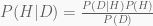
We will today just look at discrete priors. Before we can get started we have to recap the Bayes’ Theorem as that is what Bayesian Updating is based on. The Bayes’ Theorem allows us to invert conditioned probabilities:
Three Coin Problem
Suppose we have 4 coins of 3 types in a drawer. Two are fair and two are bend. The types A, B, C have probabilities for tails of 0.5, 0.6 and 0.9, respectively. I take a coin out of the drawer and flip it. The result is tails. What is the probability of a A, B, C type coin? Or in mathematical terms, what is:


Priors
Priors are the prior probabilities for the hypotheses. In or case A, B, C. Our priors are:


That is because we have a total of four coins in the drawer of which are two type A one type B and one type C.
Likelihood
The likelihood is the probability that a coin lands tails. Our likelihoods are:


Posterior
The posterior probability is the probability after we updated the prior probabilities, so the probabilities for each hypothesis given the data.
Our posteriors are:


We can see that a type A coin is still the most likely even though it lost some of its probability.
Bayesian Updating Tables
We can organise the whole updating process in a table:
| Hypothesis | Prior | Likelihood | unnormalised Posterior | normalised Posterior |
| H | P(H) | P(D|H) | P(D|H)P(H) | P(H|D) |
| A | 0.5 | 0.5 | 0.25 | 0.4 |
| B | 0.25 | 0.6 | 0.15 | 0.24 |
| C | 0.25 | 0.9 | 0.225 | 0.36 |
| Total | 1 | 0.625 | 1 |
The total of the unnormalised posterior column is P(D).

The hypothesis H is often denoted 
Updating again and again
Of course we want to update again and again and don’t worry that is easier than you might think. The posterior from before just becomes the new prior. We therefore get the following expression in the unnormalised posterior column:

That’s all.
We will soon do some experiments involving Bayesian Updating, so we can deepen our understanding and do some practical work and not just try to remember things or stick to the theoretical part.
